Specification in Multiple Regression

Moving forward with our discussion of statistical elaboration we turn now to discuss specification or interaction. Among psychologists this is also known as moderation. We use this when we think two variables work together to produce a particular effect. For example, one might theorize that political ideology and political interest work together to influence attitudes toward recreational marijuana use. 

Here is a graphic illustrating specification:
https://www.dataart.ca/wp-content/uploads/2022/05/Complete-Specification-1.pdf

In SPSS we can do this by computing an interaction term. And this is done using a compute command (e.g.compute interact= (x₁ * x₂)). 

compute interact= (x₁ * x₂)

Great care must be taken to ensure that interaction terms are correctly computed. Let’s concentrate on their calculation and then their presentation shortly.

An interaction term and the two independent variables of which it is composed must all be entered into the regression equation. Leaving out any of the constituent variables can produce misleading results.

In addition to using dummy variables, interaction terms can be computed using ordinal or interval level data but one has to be very sure what we are getting by looking closely at what we are multiplying together and what we are getting as a product.

Consider this:

	(0)	(.5)	(1)
(0)	0	0	0
(.5)	0	.25	.5
(1)	0	.5	1

And:

	(1)	(2)	(3)
(1)	1	2	3
(2)	2	4	6
(3)	3	6	9

Both of these produce valid interaction terms.

One can also use two dummy variable to compute an interaction term, but it is essential to ensure that in multiplying your dummy variables together you obtain a value of 1 only for the category of interest to you. For example, based on our previous work we might expect that being both female and Hispanic will make someone even less supportive of the marijuana initiative than each separate effect. The following coding will produce an interaction term with which to examine this hypothesis.
compute FemHisp = Female*Hisp.

	Male    (0)	Female (1)
Non- Hispanic (0)	0	0
Hispanic (1)	0	1

Unfortunately, this hypothesis turns out not supported in the analysis. Numerous other interactions with dichotomous variables in the 2016 PPIC data set also failed to produce significant effects in predicting RawMJ3.

One should be particularly careful not to use one dummy and an ordinal variable in creating an interaction term.

variable codings	(0)	(1)
(0)	0	0
(.5)	0	.5
(1)	0	1

You will note that the interaction term (in the far right column) is perfectly correlated with the ordinal variable coding (in the far left column).

Interaction or specification models contain at least one independent variable that is created by multiplying together two or more of the other independent variables. This allows us to test theories about how the effects of one independent variable on our dependent variable may be contingent upon the value of another independent variable.

Some interaction effects do appear in the PPIC 2016 data using ordinal variables. One is between ideology and interest. This is explored below using regression using the following interaction term:

compute libint = (liberal5 * interest).

Calculating the Interaction Term

                                    Ideology (liberal5)

very consev conservative neither liberal very liberal

Interest	(0)	(.25)	(.5)	(.75)	(1)
(0) low	0	0	0	0	0
(.33)	0	.0825	.165	.2475	.33
(.66)	0	.165	.33	.495	.66
(1) hi	0	.25	.5	.75	1

You will note this is very similar to the interaction term calculation for two dichotomies.

Predicting Support for Recreation Marijuana (RawMJ3) with Political Ideology (liberal5), Political Interest (Interest) and their interaction. (Standardized Coefficients)

		Model 1	Model 2	Model 3
	liberal5	360***	.366***	.136
	interest		.139***	-.011
	libint			.285**
Adj R2		.129	.147	.155
N =		(980)	(980)	(980)

Source: Oct 2016 PPIC data

*Interaction Syntax*.

compute libint = (liberal5 * interest).

regression variables=RawMJ3 liberal5 interest libint
   /statistics anova coeff r tol
   /descriptives = n
   /dependent = RawMJ3
   /method = enter liberal5
   /method = enter interest
   /method = enter Libint.

Here’s a more detailed version of the output:

Regression of RawMj3 on Ideology, Interest and their Interaction

Model		b	std err	Beta	t	sig	tol
1	Constant	.834	.067		12.5	.000
	liberal5	1.350	.112	.360	12.1	.000	1.000
2	Constant	.440	.107		4.1	.000
	liberal5	1.371	.111	.366	12.4	.000	.998
	interest	.572	.121	.139	4.7	.000	.998
3	Constant	.890	.178		4.9	.000
	liberal5	.510	.295	.136	1.7	.084	.139
	interest	-.045	.230	-.011	-.2	.846	.275
	libint	1.191	.379	.285	3.1	.002	.105

Source: Oct 2016 PPIC data. N=960.
R-square Model 1 = .129; Model 2 =.147; Model 3 = .155.

The positive coefficient for the interaction term (libint) tells us that liberals who are politically interested show more support for recreational marijuana use. However there are numerous problems of interpretation of regression results using interaction terms.

1. It is very difficult to interpret the constituent parts of the interaction, in this case liberal5 and interest. Both their coefficients have changed markedly in Model 3.
2. Moreover, the variables used to compose the interaction can become insignificant. In this case, both liberal5 and interest are no longer significant in Model 3.
3. Tolerances can go haywire. All three of the terms in Model 3 have troubling tolerances indicating issues of collinearity. This makes sense since the interaction term is composed of the other predictors in the equation.

There are some ways to handle these problems, but only the graphic approach is covered here. A mathematical approach entails centering the simple predictors (IVs) around their means. We will discuss this in class as time permits.

The graphic approach entails plotting the predicted values for the dependent variable using the regression equation.

With five categories for ideology and four for Interest we have 5X4 or 20 possible versions of the equation, but we need only to plot the results using the extreme high and low values of the variables.

                                                   constant + liberal5 + interest + libint

(Lib & Hi Int)    =  .890 (1) + .510 (1)  -.045 (1) + 1.91 (1) = 2.546
(Lib & Lo Int)   =  .890  (1) + .510 (1) -.045 (0) + 1.91 (0) = 1.400

(Cons & Hi Int) =  .890 (1) + .510 (0) -.045 (1) + 1.91 (0) =  .845
(Cons & Lo Int) = .890 (1) + .510 (0) -.045 (0) + 1.91 (0) =  .890

These values can be plotted either by hand or using Excel or a similar program.

In Excel enter:

	Conservative	Liberal
Low interest	.890	1.400
high interest	.845	2.546

Here’s the resulting Excel graphic:

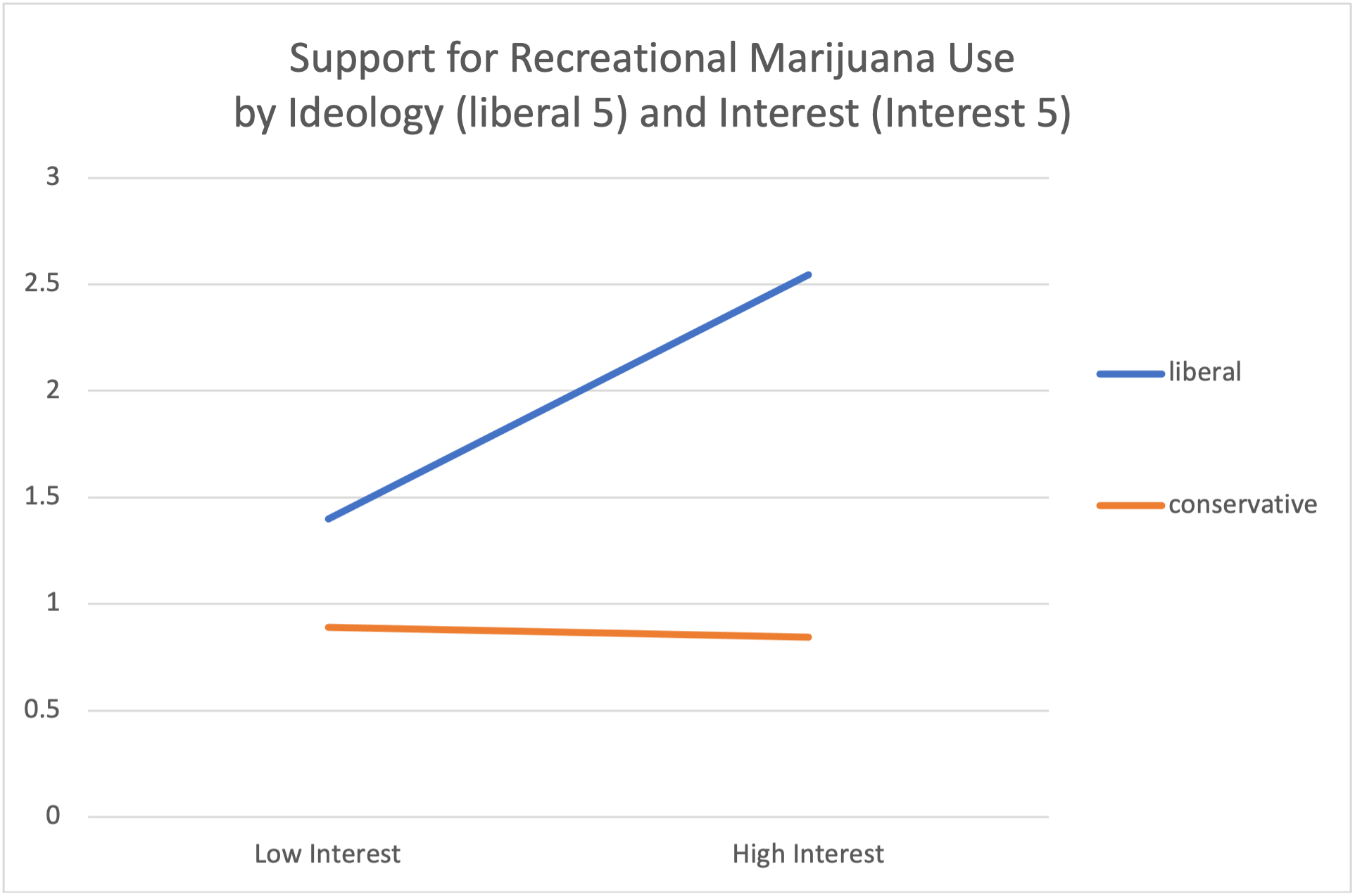
Source: PPIC October 2016

This graphic specifies the conditions under which political ideology and political interest combine (interact) to increase support for recreational marijuana use. The upper line shows that liberal respondents who are high in interest are more likely to support recreational marijuana usage than are liberals with low interest. And the lower line indicates that conservative support for recreational use of marijuana remains low irrespective of political interest.

In short, the slope for liberals is greater than for conservatives. Depicting such non-parallel lines is a typical way to illustrate specification or interaction. This is also sometimes called moderation by psychologists.

Partial as well as complete specification is possible. This is to say that there may be some remaining direct effects of the constituent variables on the dependent variable. This occurs when the constituent variables remain statistically significant in the equation.

To assess these direct effects we need to make sense of the b or Beta coefficients for the constituent variables. To do so requires a more mathematical approach.

But conceptually, we can perhaps illustrate the distinction between complete and partial specification using arrow diagrams.

This graphic approach moves us some distance along the way to building more complex path models. This topic will be introduced as time permits.