ANOVA (One-Way)                          

PURPOSE

• Understand the null hypothesis in terms of Type I and Type II errors
• Learn how to perform and interpret an ANOVA test for significance
• Learn how to interpret confidence intervals
• Gain further insight into results of crosstabulations

MAIN POINTS

Types of Error, the null hypothesis and statistical significance

• Researchers often distinguish Type I and II errors.
• Type I occurs when we conclude that there is a relationship between two variables when there is actually none (a false positive).
• Type II occurs when we conclude that there is no relationship between two variables when one exists in reality (a false negative).

		REALITY
		No Relationship	Relationship
ANALYTICAL CONCLUSION	No Relationship	accurate	Type II Error
	Relationship	Type I Error	accurate

• Researchers routinely take the null hypothesis of no relationship between variables as the basis for their work.
• Measures of significance are used to rule out the null hypothesis and avoid making Type I errors.
• A significance or probability level indicates the percentage chance of making a Type I Error.
• Probabilities of .05 and less are conventionally taken as grounds for ruling out the null hypothesis and concluding a relationship does exist.

One-way ANOVA

• One-way ANOVA:  ANalysis Of VAriance.
• One-way Anova is used to see whether the mean of the dependent variable differs across categories of an independent (group) variable.
• The independent variable used in an ANOVA test can have 3 or more categories and may be nominal or ordinal.  The dependent variable is ideally an interval variable.
• Anova can also be used with an ordinal dependent variable, particularly one with many values such as we have using an un-recoded (raw) index.
• Anova produces an F statistic which measures the ratio of between-group variation to within-group variation.
• The higher the value of F, the more likely the difference between the means is significant, i.e., not due to chance.
• An F score is compared to a probability distribution to arrive at the probability (p) value.
• Probability levels for F are interpreted in the same way as those for Chi-square.

EXAMPLE #1 — Conventional Use of ANOVA

• Dataset:
  • PPIC October 2016

• Dependent Variable:
  • Raw Index of Support for Recreational Marijuana                (7 categories coded 0-3)
• Independent Variables:
  • Partisan Identification
  • Political Ideology
• Hypotheses Arrow Diagrams:
  • H1: Democratic Party ID → Support Recreational Marijuana (7 categories coded 0-3)
  • H2: Liberal Ideology → Support for Recreational Marijuana (3 categories coded 0-3)

• Syntax

*Weighting the Data*.
weight by weight.
*Recoding MJ Index Items*.
recode q21 (1=1) (2=0) into MJPropD.
value labels MJPropD 1 'yes' 0 'no'.
recode q36 (1=1) (2=0) into MJLegalD.
value labels MJLegalD 1 'yes' 0 'no'.
recode q36a (1=1) (2=.5) (3=.0) into MJTry.
value labels MJTry 1 'recent' .5 'not recent' 0 'no'.

*Constructing an Index with alpha = .777*.
compute RawMJ3 = (MJPropD + MJLegalD + MJTry).

*Recoding the Index-Not used in this section*.
*recode RawMJ3 (0, .5=0) (1 thru 2= .5) (2.5, 3 =1) into MJ3*.
*value labels MJ3 0 'low' .5 'med' 1 'hi'*.

*Creating IV Indicators of Party Identification & Ideology*.
recode q40c (1=0) (3=.5) (2=1) into Democrat.
value labels Democrat 1 'Democ' .5 'Indep' 0 'Repub'.
recode q37 (1,2=1) (3=.5) (4,5= 0) into liberal3.
value labels liberal3 1 'liberal' .5 'middle' 0 'conserv'.

*One-way ANOVA for H1*.
oneway RawMJ3 by Democrat
  /statistics=descriptives
  /ranges=scheffe
  /plot means.

*One-way ANOVA for H2*.
oneway RawMJ3 by Liberal3
  /statistics=descriptives
  /ranges=scheffe
  /plot means.

• Syntax Legend
  • Missing values and recodes are specified as usual
  • Each oneway (anova) command lists the raw (un-recoded) DV followed by relevant IV
  • The optional /ranges=scheffe subcommand produces a table indicating which groups differ significantly
  • The optional /plot means command produces a graphic showing the mean score on the DV for each group defined by the IV.

H1 Output

Descriptives

Descriptives
RawMJ3 by Partisanship
	N	Mean	Std. Deviation	Std. Error	95% Confidence Interval for Mean
					Lower Bound	Upper Bound
Repub	230	.9705	1.08721	.07173	.8292	1.1118
Indep	370	1.7714	1.10933	.05763	1.6581	1.8847
Democ	369	1.5978	1.11807	.05822	1.4833	1.7123
Total	969	1.5154	1.14983	.03694	1.4429	1.5879

ANOVA
RawMJ3
	Sum of Squares	df	Mean Square	F	Sig.
Between Groups	94.998	2	47.499	38.724	.000
Within Groups	1184.906	966	1.227
Total	1279.904	968

Multiple Comparisons
Dependent Variable:   RawMJ3
Scheffe
(I) Democrat	(J) Democrat	Mean Difference (I-J)	Std. Error	Sig.	95% Confidence Interval
					Lower Bound	Upper Bound
Repub	Indep	-.80089*	.09300	.000	-1.0289	-.5729
	Democ	-.62725*	.09308	.000	-.8554	-.3991
Indep	Repub	.80089*	.09300	.000	.5729	1.0289
	Democ	.17364	.08147	.104	-.0261	.3734
Democ	Repub	.62725*	.09308	.000	.3991	.8554
	Indep	-.17364	.08147	.104	-.3734	.0261
*. The mean difference is significant at the .050 level.

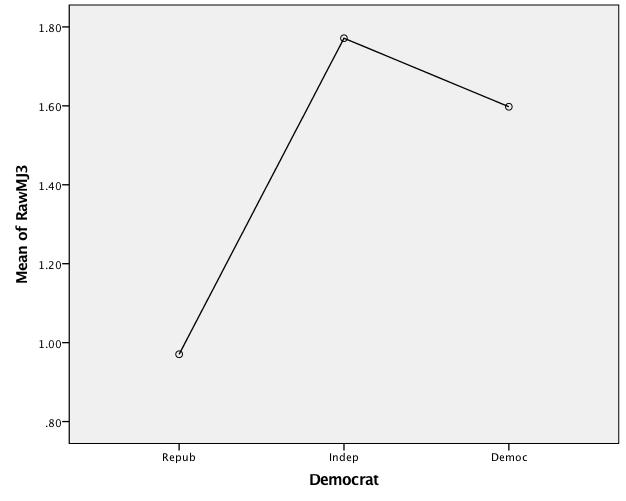
  Means Plot RawMJ3 By Partisanship

• H1 Interpretation

• • The Descriptives panel shows the mean scores on the DV (ranging from 0-3) for each category of the IV. Thus Republicans score just under 1 while Independents and Democrats score a bit over 1.5. In addition information is provided regarding the confidence intervals around each of the means and their calculation. For Republicans the 95% confidence interval ranges from .83 to 1.1. Note that its upper boundary  does not meet the lower boundary for either Independents or Democrats, indicating that Republicans score significantly lower than either of the other groups. Note also that the lower bound for Independents is above the lower bound for Democrats, indicating that these two groups do not differ significantly (beyond what one might expect due to sampling error).
  • The ANOVA panel contains the F-score and its associated significance level for the overall analysis. The .000 significance reported here means that there is less than a 1 in 1000 chance that the observed mean differences on the Recreational Marijuana index are due simply to sampling error. Thus, there is a significant difference in attitudes toward marijuana across partisan groups. However, this panel does not indicate where such differences may be.
  • The Multiple Comparisons panel calculates the mean difference between each pair of groups and uses information from the Descriptives panel to calculate which pairs of groups differ significantly from one another. Look closely at the Mean Difference (3rd from left) column. Asterisks indicate pairwise comparisons which significantly differ. Where there is no asterisk, the groups do not differ significantly. In this case, Democrats and Independents do not significantly differ but Republicans differ significantly from both Democrats and Independents. This confirms what can be observed in the Descriptives panel.
  • The Means Plot provides a graphic depiction of the mean differences in attitudes regarding recreational marijuana across the partisan groups. In this case, the plot confirms that there is not an ordered relationship between the IV and DV because while support for recreational marijuana increases in moving from Republican to Independent partisanship, it does not again increase from Independent to Democratic partisanship.

H2 Output

Descriptives
RawMJ3 by Ideology

	N	Mean	Std. Deviation	Std. Error	95% Confidence Interval for Mean
					Lower Bound	Upper Bound
conserv	335	1.0301	1.12000	.06120	.9098	1.1505
middle	288	1.6116	1.12250	.06619	1.4814	1.7419
liberal	359	1.9152	1.03832	.05483	1.8074	2.0231
Total	981	1.5241	1.15359	.03683	1.4518	1.5964

ANOVA
RawMJ3
	Sum of Squares	df	Mean Square	F	Sig.
Betw Groups	138.777	2	69.389	58.227	.000
Within Groups	1165.479	978	1.192
Total	1304.256	980

Multiple Comparisons
Dependent Variable:   RawMJ3
Scheffe
(I) liberal3	(J) liberal3	Mean Difference (I-J)	Std. Error	Sig.	95% Confidence Interval
					Lower Bound	Upper Bound
conserv	middle	-.58151*	.08776	.000	-.7966	-.3664
	liberal	-.88509*	.08296	.000	-1.0885	-.6817
middle	conserv	.58151*	.08776	.000	.3664	.7966
	liberal	-.30358*	.08641	.002	-.5154	-.0917
liberal	conserv	.88509*	.08296	.000	.6817	1.0885
	middle	.30358*	.08641	.002	.0917	.5154
*. The mean difference is significant at the .050 level.

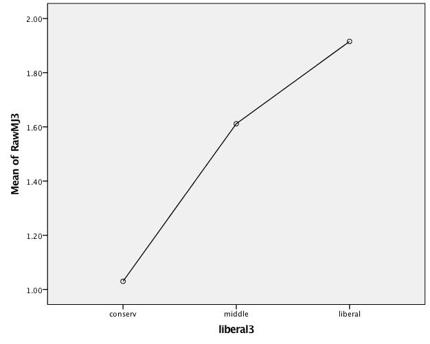
Means Plot of RawMJ3 Index Scores by Ideology

• H2 Interpretation

• • The Descriptives panel shows the mean scores on the DV (ranging from 0-3) for each category of the IV. Thus conservatives score just over 1 while liberals score just under 2, with the middle group at 1.6. Additional information on confidence intervals shows that none of the confidence intervals overlap, indicating that all three groups differ significantly (beyond what one might expect due to chance).
  • The ANOVA panel contains the F-score and its associated significance level for the analysis. It shows there are significant differences in attitudes across the ideological groups, but does not indicate where these may be.
  • The Multiple Comparisons panel calculates the mean difference between each pair of groups The Mean Difference (3rd from left) column again uses asterisks indicate pairwise comparisons which significantly differ.  In this case, all three ideological groups differ, confirming what can be observed in the Descriptives panel.
  • The Means Plot provides a graphic depiction of the mean differences in attitudes regarding recreational marijuana across the ideological groups. In this case, the plot confirms that there is an ordered relationship between the IV and DV because support for recreational marijuana increases in moving from conservative to middle of the road and increases again moving from middle of the road to liberal ideology.

• INSTRUCTIONS

1. Using your index from Lab 9, hypothesize a relationship between it and an independent variable.
   1. For example, lenient attitudes toward immigration should increase with education.
   2. The independent (group) variable should have three or more categories and be either nominal, or ordinal.
   3. The dependent variable should ideally be interval, although you can use an ordinal variable with multiple categories. Hence an index such as you constructed will work fine.
   4. Make Frequency runs for each of the variables to identify missing values and recodes.
   5. Perform a One-way ANOVA
      1. specify the DV first, then the IV
      2. include a statistics subcommand for descriptives
      3. request a scheffe test on the ranges subcommand
      4. ask for means to be plotted.
   6. Based on the output, determine whether differences in means on the dependent variable across the categories of the independent (group) variable are likely due to sampling error, or are representative of the population. Make this judgment using the .05 significance level.
   7. Repeat the steps above until you find a pair of variables (a DV and IV) that yield significant results for the ANOVA test.

QUESTIONS FOR REFLECTION

• Did you find a significant result? If so, what is the likelihood that you are making a Type I Error?
• How does One-way ANOVA differ from a chi-square?

DISCUSSION

• Recall that the measure of significance represents the likelihood of making a Type I error.  So if sig.=.03, then the likelihood that you are making a Type I error (concluding there is a relationship, when there is none) is 3 in 100. If your sig. or p=.000, the chances of a Type I error is less than 1 in a thousand.
• The chi-square assesses significance in a crosstabulation. ANOVA compares mean scores across categories of the independent variable. For this the DV should be measured at the interval level or at the ordinal level when there are a substantial number of categories, as is the case with a summary index.

FURTHER TECHNICAL DETAILS (optional)

• The F-score is calculated as the ratio of between group to within group  figures in Mean Square column of the Anova table. Thus on H1 a between group variance of 47.499 divided by a within group variance of 1.227 = 38.7. This figure is compared to a sampling distribution for F-scores to determine significance. It indicates the number of standard deviations this difference lies from the mean of the sampling distribution. Since roughly two standard deviations (1.96) comprise 95% of the cases, it forms the cut off for the .05 significance level. The F-score for H1 exceeds 38 and thus easily passes significance at the .05 and .01 level for the appropriate degrees of freedom.
• Standard Errors = square root of the variance divided by the square root of n (the number of cases for the group). Remember: variance = SD² .
•  The 95% CI for Mean column is calculated by subtracting and adding the 1.96 times the standard error to/from the mean score.
• Derivation of the Sum of Squares and Mean Squares will be discussed later in the term in connection with regression and, if there is time, two-way Anova.

EXAMPLE #2 — Extending the Use of ANOVA

USING ANOVA WITH CROSSTABS:

1. After finding a significant relationship in a crosstabulation using Chi-square, it is often also useful to consider which specific columns differ.
2. A one-way ANOVA provides an efficient approach.
3. Technically, ANOVA should be used with a dependent variable measured at the interval level or perhaps with an ordinal level variable with many values such as an index.
4. So while you might use the un-recoded version of an index as a dependent variable with ANOVA, you normally would not use an index in its recoded (two, three or four-category) form.
5. Nevertheless using a recoded form of the dependent variable in an Analysis of Variance will offer some insight as to where significance differences lie in a crosstabulation using the same variables.

INSTRUCTIONS: (Example #2 )

1. After you have found a significant relationship using crosstabulation, try a one-way ANOVA with the same pair of variables coded as they are for crosstabulation.
2. Make sure that your dependent variable is at least ordinal, as is typically the case with a recoded index.
3. Using a dependent variable recoded into several categories for a crosstabulation, Analysis of Variance will offer insight as to where the significance differences are in the crosstab.
4. Be sure to include the Scheffe test for interpretive ease.

ANOVA with recoded data (similar to crosstabulation)

• Dataset:
  • PPIC 2016
• Independent Variables:
  • Partisan Identification
  • Political Ideology
• Dependent Variable:
  • Support for Recreational Marijuana (Recoded into 3 categories, coded 0-.5-1))
• Hypothesis Arrow Diagram:
  • Democrat → Support for Recreational Marijuana (3 categories)
  • Liberal → Support for Recreational Marijuana (3 categories)

• Syntax (in addition to the syntax used above)

*Recoding the Index*.
recode RawMJ3 (0, .5=0) (1 thru 2= .5) (2.5, 3 =1) into MJ3.
value labels MJ3 0 'low' .5 'med' 1 'hi'.

oneway MJ3 by Democrat 
   /statistics = descriptives 
   /ranges=scheffe 
   /plot means.

oneway MJ3 by liberal3
   /statistics = descriptives
   /ranges=scheffe
   /plot means.

• Syntax Legend
  • Note that the DV in each case is recoded into 3 categories just as it was for the crosstabulation in Lab 10
  • Each oneway (anova) command lists the DV and one of the IVs.
  • The /statistics, /ranges and /plot subcommands produce much useful information.
    • Note again that the recoded form of the index is used here.
    • The IV takes on the same values as in the Crosstab.

• H1 Output
  Descriptives
  MJ3 (0, .5, 1) by Democrat

	N	Mean	StdDev	StdErr	95% Conf Interval
					Lower	Upper
Repub	230	.3097	.39488	.02605	.2584	.3610
Indep	370	.5800	.41703	.02167	.5373	.6226
Democ	369	.5336	.41083	.02139	.4916	.5757
Total	969	.4982	.42288	.01358	.4716	.5249

ANOVA
MJ3 (recoded)
	Sum of Squares	df	Mean Square	F	Sig.
Betw Groups	11.104	2	5.552	33.105	.000
Within Groups	162.013	966	.168
Total	173.118	968

Multiple Comparisons
Dependent Variable:   MJ3
Scheffe
(I) Democrat	(J) Democrat	Mean Difference (I-J)	Std. Error	Sig.	95% Confid Interval
					Lower	Upper
Repub	Indep	-.27027*	.03439	.000	-.3546	-.1860
	Democ	-.22394*	.03442	.000	-.3083	-.1396
Indep	Repub	.27027*	.03439	.000	.1860	.3546
	Democ	.04633	.03012	.307	-.0275	.1202
Democ	Repub	.22394*	.03442	.000	.1396	.3083
	Indep	-.04633	.03012	.307	-.1202	.0275
*. The mean difference is significant at the .050 level. Mean Plot MJ3 (recoded in 3 categories) by Democrat

• 
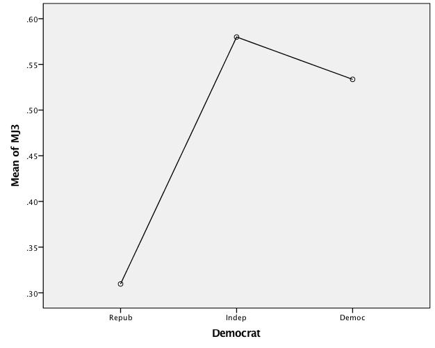
  H1 Interpretation
  • • The results are similar to those in Example 1 which used the raw (un-recoded) index for the DV
    • Here, however the DV has been recoded into three values, just as in the Crosstabulation in Labs 10 & 11. Hence the range of values is for the DV is now 0-1.
    • In each of the output panels the mean scores and confidence intervals reflect the 0-1 range of the recoded DV.
    • Again we find that Republicans differ significantly from both Independents and Democrats while Independents and Democrats do not differ significantly.
    • This provides us with information as to where the significant differences lie which is not available using Chi-square.
• H2 Output
  

  	N	Mean	StdDev	StdErr	95% Confid Interval
  					Lower	Upper
  conserv	335	.3241	.41008	.02241	.2801	.3682
  middle	288	.5273	.41126	.02425	.4795	.5750
  liberal	359	.6438	.38537	.02035	.6038	.6838
  Total	981	.5005	.42342	.01352	.4740	.5270

ANOVA
MJ3
	Sum of Squares	df	Mean Square	F	Sig.
Between	17.985	2	8.993	55.757	.000
Within	157.731	978	.161
Total	175.716	980

Multiple Comparisons
Dependent Variable:   MJ3
Scheffe
(I) liberal3	(J) liberal3	Mean Difference (I-J)	Std. Error	Sig.	95% Confidence Interval
					Lower Bound	Upper Bound
conserv	middle	-.20313*	.03228	.000	-.2823	-.1240
	liberal	-.31965*	.03052	.000	-.3945	-.2448
middle	conserv	.20313*	.03228	.000	.1240	.2823
	liberal	-.11652*	.03179	.001	-.1945	-.0386
liberal	conserv	.31965*	.03052	.000	.2448	.3945
	middle	.11652*	.03179	.001	.0386	.1945
*. The mean difference is significant at the .050 level.

Means Plot MJ3 (coded 0, .5, 1) by Ideology (liberal3)

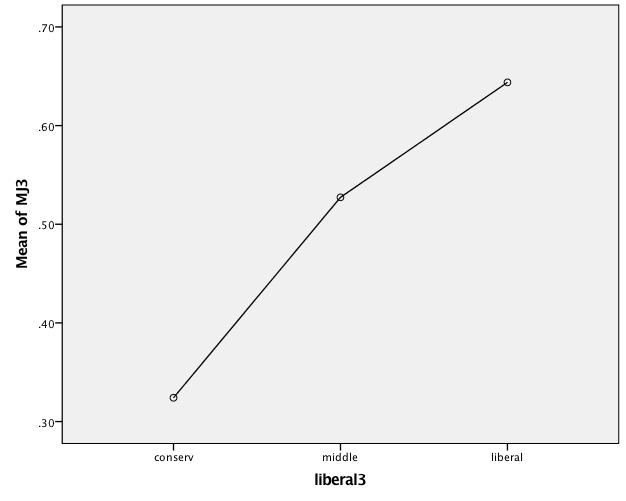
• H2 Interpretation
• Note that the DV is recoded into 3 categories as it was for crosstabulation.
• Hence the means and confidence intervals are scored 0. .5, 1.
• The results are interpreted as previously
• Comparing the Means Plots for H1 & H2 makes it clear why the ordinal relationship for H1 is weaker than that for H2 as found in Crosstabulation and the tau ordinal measure of association

QUESTIONS FOR REFLECTION

• Should the results of the one-way ANOVA lead us to rethink, or reconceptualize, the relationship between partisanship and attitude to recreational marijuana?
• How might you further use this approach?

DISCUSSION

• Chi-square can tell us whether or not there are significant differences in a cross tabulation, but chi-square alone cannot tell us where those significant differences lie. These results suggest that we might think in terms of Republican opposition to recreational marijuana instead of Democratic support. In such situations where specific differences are theoretically interesting, we can use one-way ANOVA to examine the data further and more finely tune our findings.
• Consider the relationship between MJ3 and education. The syntax for education is in Labs 7 & 11. Here is the means plot:

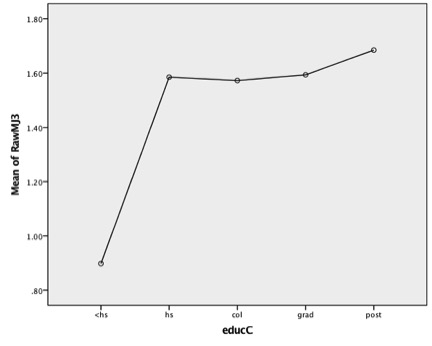
• This and the accompanying statistics suggest reformulating the hypothesis that Educ → MJ3 should be reconsidered and re-conceptualized.