
Lab 21
POL242 LAB MANUAL: Lab 21
Interpreting Interaction Terms
PURPOSE
- To learn to interpret regression results with interaction effects.
- To learn to present interaction effects in table form
MAIN POINTS
- As shown in the previous lab, elaboration patterns of specification can be incorporated into regression analysis using interaction terms.
- The presence of an interaction term is indicated in a regression equation by the introduction of a new multiplicative term that takes the form of X1X2. Thus the equation becomes y = a + bX1 + bX2 + bX1X2
- An insignificant interaction term should normally be excluded from the equation. The results in the previous lab were presented for illustrative purposes only.
- A significant interaction indicates that the independent variables X1 and X2 do not have consistent effects. Instead, the effect of each independent variable is influenced by the other independent variable.
- For instance, if we had found a significant interaction between partisanship and gender in the previous lab, this would suggest that the influence of partisanship on egalitarianism is different for males and females. Similarly the influence of gender on egalitarianism would differ across partisan groupings.
- A more complex example of significant three-way interaction between partisanship, gender and improved finances is presented below.
- In a regression model that contains a significant interaction term, the regression plane is essentially warped, with different values of b at different points along the edges of the warped plane. In the context of a significant interaction term, it is therefore essential to interpret the coefficients for the effects of X1 and X2 with exceptional care.
- Where there is a significant interaction in a regression equation, the interpretation of the coefficients for the variables included in the interaction is often facilitated by ‘centering’.
- To ‘centre’ a variable, the relevant mean value is subtracted from each score on the variables to create transformed variables, representing deviations from the mean.
- When the variables are ‘centred’ in this way, the regression coefficients show the effects of one unit change in X1 at the mean for X2 and vice versa.
- Although not its primary purpose, centering also reduces multi-collinearity in a regression equation.
- The results of an interaction analysis can perhaps best be presented in the a table showing the results of the equation using centered variables
EXAMPLE (3-way interaction)
- Dataset:
- CES2011
- Hypotheses:
- BETTER FINANCES*CONSERVATIVE*MALEà EGALITARIANISM
- Regression Syntax
weight by WGTSamp.
*Preparing indicators of Attitudes re Inequality*.
*declare missing values on pes11_41*.
missing values pes11_41 (8,9).

*reverse scoring on pes11_41 and make it range from 0-1*.
recode pes11_41 (1=1) (2=.75) (3=.5) (4= .25)
    (5=0) into undogap.
value labels undogap 0 'muchless' .25 'someless' .5 'asnow'
    .75 'somemore' 1 'muchmore'.

*rescale mbs11_k2 from 0-10 to 0-1 and reverse its scoring*.
missing values mbs11_k2 (-99).
compute govact = (((mbs11_k2 * -1) +10)/10).
value labels govact 0'not act' 1 'gov act'.

*recode and re-label mbs11_b3 and pes11_52b*.
recode mbs11_b3 (1=1) (2=0) into goveqch.
value labels goveqch 1 'decent living' 0 'leave alone'.

*create an indexed variable (alpha=.66).
compute rawegal = undogap + govact + goveqch.

*interval measure of partisan feeling from Lab 7*.
recode cps11_18 (0=0) (else = copy) into ConFeel.
missing values Confeel (996, 998, 999).

*Create gender indicator from lab6*.
recode rgender11 (1=0) (5=1) into female.
recode rgender11 (1=1) (5=0) into male.*create finance measures (from Lab 7.
missing values cps11_66 (8,9).
recode cps11_66 (1=1) (3=0) (5=.5) into finances.
variable labels finances 'personal finances'.
value labels finances 0 'worse' .5 'same' 1 'better'.*Create dummies for Finances*.
recode finances (0 = 1) (else = 0) into worse.
recode finances (.5 =1) (else = 0) into same.
recode finances (1=1) (else = 0) into better.

*Preparing IV indicator-party identification from Lab 13*.
recode cps11_71 (2=1) (1=2) (4=3) (3=4)into PID4.
value labels PID4 1 'Cons' 2 'Lib' 3 'BQ' 4 'NDP'.

*Create dummies or PID*.
recode PID4 (1=1) (else=0) into Cons.
recode PID4 (2=1) (else=0) into Lib.
recode PID4 (3=1) (else=0) into BQ.
recode PID4 (4=1) (else=0) into NDP.

*Compute interaction terms*.
compute ConsBetter = Cons*better.
compute BetterMale = better*male.
compute ConsMale = Cons*male.
compute BetterConsMale = Better*Cons*male.
fre var = BetterConsMale.

Regression variables = rawegal male worse better Cons BQ NDP
   ConsMale   ConsBetter BetterMale BetterConsMale
   /statistics coeff r tol anova
   /descriptives = n
   /dependent = rawegal
   /method = enter male Cons BQ NDP
   /method = enter ConsMale
   /method = enter worse better
   /method = enter ConsBetter
   /method = enter BetterMale
   /method = enter BetterConsMale.

*Compute centered variables*.
fre var male cons BQ NDP worse better
   /statistics mean.
*centering predictors around mean scores*.
compute Cmale = (male - .448).
compute Ccons = (Cons - .259).
compute Cbq = (BQ - .084).
compute Cndp = (ndp - 107).
compute Cworse = (worse - .210).
compute Cbetter = (better - .164).
compute CConsBetter = CCons*Cbetter.
compute CBetterMale = CBetter*Cmale.
compute CConsMale = CCons*Cmale.
compute CBetterConsMale = CBetter*CCons*Cmale.
fre var = CBetterConsMale.

Regression variables = rawegal Cmale Cworse Cbetter CCons CBQ CNDP
    CConsMale CConsBetter CBetterMale CBetterConsMale
   /statistics coeff r tol anova
   /descriptives = n
   /dependent = rawegal
   /method = enter Cmale CCons CBQ CNDP
   /method = enter CConsMale
   /method = enter Cworse Cbetter
   /method = enter CConsBetter
   /method = enter CBetterMale
   /method = enter CBetterConsMale.
- Syntax Legend
- In addition to the usual recodes a set of two-way interaction terms and a three way interaction term are constructed and used in the first regression procedure.
- Centered versions of each of the variables used in the analysis are computed by subtracting the mean score from the value of each variable.
- A second regression is run utilizing the centered variables.
Graphic Display of the Interaction
Egalitarian Attitudes by Gender, Party and Financial Circumstances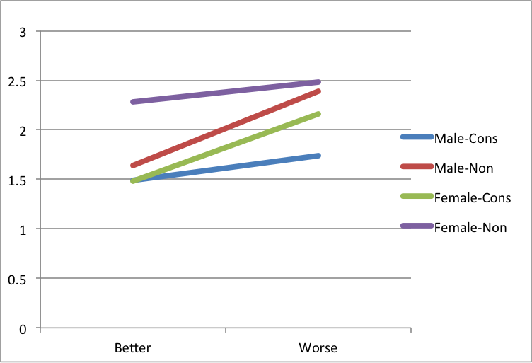
Tabular Presentation of Variables
| Statistics | |||||||
| male | Cons | BQ | NDP | worse | better | ||
| N | Valid | 3462 | 3462 | 3462 | 3462 | 3462 | 3462 |
| Missing | 0 | 0 | 0 | 0 | 0 | 0 | |
| Mean | .4480 | .2591 | .0837 | .1071 | .2101 | .1638 | |
Tabular Presentation of Regression Results
Predicting Egalitarianism by Gender and Partisanship Unstandardized Coefficients
| Model IV | tolerance | Model IV- Centered | tolerance | ||
| b (se) | b (se) | ||||
| Male (dummy) | -.068(.054) | .622 | -.154***(.043) | .972 | |
| Conserv | -.304***(.075) | .398 | -.459***(.051) | .862 | |
| BQ | .160*(.079) | .934 | .160*(.079) | .934 | |
| NDP | .164**(.067) | .912 | .164**(.067) | .912 | |
| ConsMale | -.260*(.107) | .331 | -.160(.096) | .963 | |
| Worse | .161**(.054) | .931 | .161**(.054) | .931 | |
| Better | -.021(.070) | .294 | -.203***(.062) | .857 | |
| ConsBetter | -.504**(.171) | .240 | -.232ms(.121) | .895 | |
| BetterMale | -.272(.151) | .262 | -.115(.122) | .895 | |
| BetterConsMale | .608**(.240) | .221 | .608**(.240) | .878 | |
| Constant | 2.297 | 19.668 | |||
| Adj R2 | .191 | .191 | |||
| N= | 851 | 851 |
ms =.056; *Signif <.05; **Signif <.01; ***Signif <.001
It may sometimes be preferable to present standardized coefficients.
Predicting Egalitarianism by Gender and Partisanship Standardized Coefficients
| Model IV | Model IV- Centered | ||
| β | β | ||
| Male (dummy) | -.049 | -.112*** | |
| Conserv | -.199*** | -.301*** | |
| BQ | .065* | .065* | |
| NDP | .079** | .079** | |
| ConsMale | -.130* | -.052 | |
| Worse | .095** | .095** | |
| Better | -.011 | -.108*** | |
| ConsBetter | -.186** | -.062ms | |
| BetterMale | -.109 | -.031 | |
| BetterConsMale | .166** | .083** | |
| Constant | 2.297 | 19.668 | |
| Adj R2 | .191 | .191 | |
| N= | 851 | 851 |
ms =.056; *Signif <.05; **Signif <.01; ***Signif <.001
Instructions
- For this exercise you should perform a multiple regression analysis with two-way interactionterm using centered variables.
- Calculate mean scores for the variables included in your interaction term.
- Compute deviation scores for each value by subtracting the mean from each value.
- Create a new variable to measure the interaction by multiplying the two centered independent variables together.
- Once you have made all necessary recodes, declared missing values and created an interaction term, enter all variables (including the variables used to create the interaction) into a multiple regressionequation with two steps, or blocks.
- Based on the output, build a table.
Discussion
To appreciate how centering facilitates the interpretation of regression results which include an interaction term it is useful to compare the results presented in the tables using centered and non-centered variable
Notice that the coefficients change considerably. These dramatic effects occur because the (uncentred) main effects included in the interaction term now have a special (and not very useful) meaning. In particular, each main effect for the uncentred variables included in the interaction describes the effect of its variable when the other variable in the interaction term takes on a value of zero.
As if these interpretive difficulties were not enough, multicollinearity also becomes something of a problem in the analysis using uncentered variables.
These difficulties are also evident in looking at standardized coefficients.
For these reasons, it is generally easier to interpret the effects of an interaction term using ‘centred’ variables.