
Lab 20
POL242 LAB MANUAL: Lab 20
Regressions with Interaction Terms
Interaction Terms
PURPOSE
- To learn how to use regression analysis to compare the effects of an independent variable on a dependent variable when a third variable takes on different values (interaction effects).
- To learn how to incorporate interaction terms in a single regression equation.
MAIN POINTS
- Elaboration patterns of replication, explanation, and interpretation, can be incorporated into regression analysis by simply entering the appropriate independent variables into the analysis.
- Elaboration patterns of specification can also be incorporated into regression analysis using interaction terms. Recall that specification is a pattern of elaboration where one variable affects the relationship between two other variables. This is also often described as an interaction effect. With interaction, the effects of one independent variable (x) on the dependent variable (y) are a function of a second independent variable (z).
- For instance, the effect of gender on income is different for different age groups
- In a regression, an interaction effect is present when the slope of the regression line changes depending on the value of a third variable.
- There are two ways to include interaction effects in regression analysis: The two methods calculate and express the interaction effect in slightly different ways.
- Method 1 is to run regressions with a subset of cases. This approach has been explored in previous labs on bivariate and multivariate regression. It follows a logic similar to that of using control tables.
- Method 2 is to include an interaction term in a single regression equation. An interaction term can be created by multiplying two variables together to create a new variable (e.g. compute interact= x * z). Great care must be taken to ensure that interaction terms are correctly computed. Generally, you want to ensure that in multiplying your dummy variables together you obtain a value of 1 only for the category or interest to you. In this case, we expect that being female and over 30 leads to lower income. So we should ensure that in our dummy variables Female =1 and over 30 =1.
- The interaction term and the two independent variables from which it is computed are all entered into a single regression equation.
- In addition to using dummy variables, interaction terms can be computed using ordinal or interval level data. Here we will focus only on dummy variables.
- The example analyzes the effects of differential effect of gender on income levels among different age groups.
EXAMPLE
- Dataset:
- CES2011
- Hypotheses Arrow Diagrams:
- [MALE] X [Conservative] –> [~Egalitarianism]
Regression Syntax
compute ConsMale = Cons*male.
Regression variables = rawegal male worse better Cons BQ NDP ConsMale
   /statistics coeff r tol anova
   /descriptives = n
   /dependent = rawegal
   /method = enter male Cons BQ NDP
   /method = enter ConsMale.
- Syntax Legend
- The usual missing values and recodes from previous labs are assumed here
- These include dummy variables for both Gender and partisanship. Unlike previous labs,in this instance Gender is recoded as Male=1 in order to create a clear hypothesis that conservative males are likely to be less egalitarian than others. Alternatively, a female*nonConservative interaction term could have been used.
- Creating the interaction term entails computing a multiplicative term combining gender and partisanship as shown in this multiplication table.
| Female (0) | Male (1) | |
| Non-Cons (0) | 0 | 0 |
| Conserv (1) | 0 | 1 |
- Be sure to include “tol” in the statistics line in order to assess multicollinearity.
- Note that two /method subcommands are included, the first without the interaction term and the second with it.
Output
The findings from the raw SPSS output has been converted to the recommended multi-model table format. Predicting Egalitarianism by Gender and Partisanship Unstandardized Coefficients
| Model I | Model II | Model III | |
| b (se) | b (se) | b (se) | |
| Male (dummy) | -.184*** (.047) | -.154***(.043) | -.131*(.051) |
| Conserv | -.508*** (.051) | -.438***(.068) | |
| BQ | .183*(.080) | .182*(.080) | |
| NDP | .177**(.068) | .179**(.068) | |
| ConservMale | -.146(.096) | ||
| Constant | 2.074 | 2.194 | 2.218 |
| Adj R2 | .017 | .158 | .159 |
| N= | 851 | 851 | 851 |
*Signif <.05; **Signif <.01; ***Signif <.001
Interpretation
- Model I contains only the bivariate relationship between gender (coded as male) and egalitarianism. The negative sign tells us that men are less egalitarian than the reference category (women). Model IIshows theadditiveeffects of gender and partisanship on level of egalitarianism..
- The mathematical interpretation of the b coefficients, the Adjusted R-square, the confidence intervals, and statistical significance is the same as described in the Regression Lab. Thus, it will not be repeated here. Note that both gender and all three of the partisan dummy variables are statistically significant.
- In addition to the effects of gender and partisanship on egalitarianism Modell III also shows the effect of the interaction of being male and conservative on egalitarianism.
- The simple gender and partisanship variables are all statistically significant, but the interaction term is not. Typically, such insignificant effects are not interpreted further and the results for the model without the interaction are reported.
- Multi-collinearity is frequently a problem in interactive regression models because the interaction term is constructed from two variables that are already included in the model. While tolerance scores should be routinely calculated as part of any regression equation, it is particularly important to do so for regressions containing an interaction term. Recall from the Lab on the Multiple Regression that tolerances scores approaching .20 may signal reason for concern and tolerance scores lower than .10 indicate a serious problem with multi-collinearity.
- A significant interaction term can be described as specification or interaction. It can perhaps be best interpreted by converting the results to a graphic (see Linneman Ch12). Although the present interaction term is not significant the elements of the procedure are as follows:
Constant + male + Conserv + ConsMale
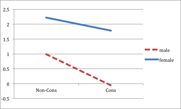
Egal (Male & Cons) = 2.22 – 1.13(1) – .44(1) – .71(1) = -0.06
Egal (Male & not Cons) = 2.22 – 1.13(1) – .44 (0) -.71(0) = 0.99
Egal (Female & Cons) = 2.22 – 1.13(0) – .44(1) – .71(0) = 1.78
Egal (Female & notCons) = 2.22 – 1.13(0) – .44(0) -.71(0) = 2.22
These results yield the following plot showing apparently (but in this case not significantly) different slopes for men and women.
Egalitarianism by Party by Gender
Instructions
- For this exercise you will perform a multiple regression analysis with an interaction term
- Create an interaction term: As always, it is best to work with an explicit hypothesis in mind.
- Multiply two independent variables together to create the interaction term.
- Create a new variable (with a new variable name) to measure the interaction. You can name it “inter” or something more descriptive.
compute inter=IndependentVar*ZVar. - Once you have made all necessary recodes, declared missing values and created an interaction term, enter all variables (including the variables used to create the interaction) into a multiple regressionequation using two or more steps, or blocks.
- regression variables=DVar IVar1 IVar2 Inter
/statistics coeff outs r tol
/dependent=DVar
/method=enter IVar1 IVar2
/method=enter Inter.
- regression variables=DVar IVar1 IVar2 Inter
- Based on the output, determine whether the dummy variables and the interaction term are significant. If neither are, repeat the process until you find an appropriate set.
DISCUSSION
- As already mentioned, the two methods for analyzing interaction effects in a regression simply express the interaction (or specification) effect in a slightly different way. But the two methods have different advantages and disadvantages:
- When you have only one interaction (specification) of interest, the regression with a subset of cases approach is often easier to use and interpret. An example of one such an interaction (specification) is geographic region: many of the relationships between independent and dependent variables differ in different parts of the world (e.g. Francophone Quebec vs. the rest of Canada; Africa versus other parts of the world).
- Regression with a subset of cases doesn’t readily allow you to examine several different kinds of interaction effects simultaneously: you may, for example, want to test not only whether gender affects the relationship between age and income, but also whether education affects the relationship between region and income. Such complex models cannot readily be analyzed using the regression with a subset of cases method. Moreover, this approach is only appropriate when the control variable has very few categories.
- The approach of including an interaction term can often be difficult to set up and to interpret. However, the interaction term approach enables you to examine a variety of different interactions simultaneously. Moreover, using this method you can directly compare the R-squares for the additive and interactive models to see whether the interaction explains more variation on y.