
Lab 12
POL242 LAB MANUAL: Lab 12
ANOVA (One-Way)
PURPOSE
- Understand the null hypothesis in terms of Type I and Type II errors
- Learn how to perform and interpret an ANOVA test for significance
- Learn how to interpret confidence intervals
- Gain further insight into results of crosstabulations
MAIN POINTS
Types of Error, the null hypothesis and statistical significance
- Researchers often distinguish Type I and II errors.
- Type I occurs when we conclude that there is a relationship between two variables when there is actually none (a false positive).
- Type II occurs when we conclude that there is no relationship between two variables when one exists in reality (a false negative).
| REALITY | |||
| No Relationship | Relationship | ||
| ANALYTICAL CONCLUSION | No Relationship | accurate | Type II Error |
| Relationship | Type I Error | accurate | |
- Researchers routinely take the null hypothesis of no relationship between variables as the basis for their work.
- Measures of significance are used to rule out the null hypothesis and avoid making Type I errors.
- A significance or probability level indicates the percentage chance of making a Type I Error.
- Probabilities of .05 and less are conventionally taken as grounds for ruling out the null hypothesis and concluding a relationship does exist.
One-way ANOVA
- One-way ANOVA: ANalysis Of VAriance.
- One-way Anova is used to see whether the mean of the dependent variable differs across categories of an independent (group) variable.
- The independent variable used in an ANOVA test can have 3 or more categories and may be nominal or ordinal. The dependent variable is ideally an interval variable.
- Anova can also be used with an ordinal dependent variable, particularly one with many values such as we have using an un-recoded (raw) index.
- Anova produces an F statistic which measures the ratio of between-group variation to within-group variation.
- The higher the value of F, the more likely the difference between the means is significant, i.e., not due to chance.
- An F score is compared to a probability distribution to arrive at the probability (p) value.
- Probability levels for F are interpreted in the same way as those for Chi-square.
EXAMPLE #1 — Conventional Use of ANOVA
- Dataset:
- CES 2011
- Hypothesis Arrow Diagram:
- Party ID → Egalitarianism
- Syntax
*Weighting the Data*.
weight by WGTSamp.

*Preparing indicators of Attitudes re Inequality*.
*declare missing values on pes11_41*.
missing values pes11_41 (8,9).

*reverse scoring on pes11_41 and make it range from 0-1*.
recode PES11_41 (1=1) (2=.75) (3=.5) (4= .25)
   (5=0) into undogap.
value labels undogap 0 'muchless' .25 'someless' .5 'asnow'
   .75 'somemore' 1 'muchmore'.

*rescale mbs11_k2 from 0-10 to 0-1 and reverse its scoring*.
missing values mbs11_k2 (-99).
compute govact = (((mbs11_k2 * -1) +10)/10).
value labels govact 0'not act' 1 'gov act'.

*recode and re-label mbs11_b3 and pes11_52b*.
recode mbs11_b3 (1=1) (2=0) into goveqch.
value labels goveqch 1 'decent living' 0 'leave alone'.

*create an indexed variable (alpha=.66).
compute rawegal = undogap + govact + goveqch.

*recode the new index into three categories*.
recode rawegal (0 thru 2.10=0)(2.15 thru 2.50=.5)
   (2.55 thru 3= 1) into egal3.
value labels egal3 0 'low' .5 'med' 1 'hi'.

*Preparing X indicator-party identification*.
recode cps11_71 (2=1) (1=2) (4=3) (3=4)into PID4.
value labels PID4 1 'Cons' 2 'Lib' 3 'BQ' 4 'NDP'.

*One-way ANOVA*.
oneway rawegal by PID4
   /statistics=descriptives
   /ranges=scheffe
   /plot means.
- Syntax Legend
- Missing values and recodes are specified as usual
- The oneway (anova) command lists the DV followed by IV
- The optional /ranges=scheffe subcommand produces a table indicating which groups differ significantly
- The optional /plot means command produces a graphic showing the mean score on the DV for each group defined by the IV.
- Output
Descriptives
| N | Mean | Std. Dev | Std. Error | 95% Confidence Interval | ||
| Lower Bound | Upper Bound | |||||
| Cons | 236 | 1.7649 | .81062 | .05272 | 1.6611 | 1.8688 |
| Lib | 213 | 2.2473 | .56600 | .03882 | 2.1708 | 2.3238 |
| BQ | 72 | 2.4585 | .40299 | .04765 | 2.3635 | 2.5535 |
| NDP | 107 | 2.4662 | .46673 | .04511 | 2.3768 | 2.5557 |
| Total | 628 | 2.1270 | .70484 | .02814 | 2.0717 | 2.1822 |
| ANOVA | |||||
| rawegal | |||||
| Sum of Squares | df | Mean Square | F | Sig. | |
| Between Groups | 54.250 | 3 | 18.083 | 43.829 | .000 |
| Within Groups | 257.045 | 623 | .413 | ||
| Total | 311.295 | 626 | |||
| Multiple Comparisons | ||||||
| Dependent Variable: rawegal | ||||||
| Scheffe | ||||||
| (I) PID4 | (J) PID4 | Mean Difference (I-J) | Std. Error | Sig. | 95% Confidence Interval | |
| Lower Bound | Upper Bound | |||||
| Cons | Lib | -.48238* | .06071 | .000 | -.6526 | -.3122 |
| BQ | -.69356* | .08668 | .000 | -.9365 | -.4506 | |
| NDP | -.70132* | .07483 | .000 | -.9111 | -.4915 | |
| Lib | Cons | .48238* | .06071 | .000 | .3122 | .6526 |
| BQ | -.21118 | .08780 | .124 | -.4573 | .0349 | |
| NDP | -.21894* | .07613 | .042 | -.4323 | -.0055 | |
| BQ | Cons | .69356* | .08668 | .000 | .4506 | .9365 |
| Lib | .21118 | .08780 | .124 | -.0349 | .4573 | |
| NDP | -.00776 | .09810 | 1.000 | -.2827 | .2672 | |
| NDP | Cons | .70132* | .07483 | .000 | .4915 | .9111 |
| Lib | .21894* | .07613 | .042 | .0055 | .4323 | |
| BQ | .00776 | .09810 | 1.000 | -.2672 | .2827 | |
| *. The mean difference is significant at the .050 level. | ||||||
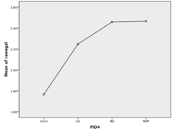
Means Plot
- Interpretation
- The Descriptives panel shows the mean scores on the DV for each category of the IV plus information on the confidence intervals around the means and their calculation.
- The ANOVA panel contains the F-score and its associated significance level for the analysis. The .000 significance means that there is less than a 1 in 1000 chance that the observed mean differences on the egalitarian index are due simply to sampling error. Thus, there is a significant difference in egalitarian attitudes across partisan groups.
- The Multiple Comparisons panel calculates the mean difference between each pair of groups and uses information from the Descriptives panel to calculate which pairs of groups differ significantly from one another.
- The Means Plot proves a graphic depiction of the mean differences in Egalitarian attitudes across Partisan groups.
INSTRUCTIONS
- Using your index from Lab 9, hypothesize a relationship between it and an independent variable
- For example, egalitarian attitudes should vary with Party Identification.
- The independent (group) variable should have three or more categories and preferably be nominal, although it can be ordinal.
- The dependent variable should ideally be interval, although you can use an ordinal variable with multiple categories.
- Make Frequency runs for each of the variables to identify missing values and recodes.
- Perform a One-way ANOVA
- specify the DV first, then the IV
- include a statistics subcommand for descriptives
- request a scheffe test on the ranges subcommand
- ask for means to be plotted.
- Based on the output, determine whether differences in the means on the dependent variable across the categories of the independent (group) variable are likely due to sampling error, or are representative of the population. Make this judgment using the .05 significance level.
- Repeat the steps above until you find a pair of variables that yield significant results for the ANOVA test.
QUESTIONS FOR REFLECTION
- Did you find a significant result? If so, what is the likelihood that you are making a Type I Error?
- How does One-way ANOVA differ from a chi-square?
DISCUSSION
- Recall that the measure of significance represents the likelihood of making a Type I error. So if sig.=.03, then the likelihood that you are making a Type I error (concluding there is a relationship, when there is none) is 3 in 100.
- The chi-square compares assess significance in a crosstabulation. ANOVA compares mean scores across categories of the independent variable. For this the DV should be measured at the interval level or at the ordinal level when there are a substantial number of categories, as is the case with an summary i
FURTHER TECHNICAL DETAILS
- The F-score is calculated as the ratio of between group to within group variances using the figures in Mean Square column of the Anova table. Thus 18.08 divided by .413 = 43.8. This figure is compared to a sampling distribution for F-scores to determine significance. It indicates the number of standard deviations this difference lies from the mean of the sampling distribution. Since roughly two standard deviations (1.96) comprise 95% of the cases, it forms the cut off for the .05 significance level. The F-score here exceeds 43 and thus easily passes significance at the .01 level for the appropriate degrees of freedom (3; 623) in Appendix C of Linneman (C-5).
- Standard Errors = square root of the variance divided by the square root of n (the number of cases for the group). Remember: variance = SD2, so for Conservatives this yields .81/15.4=.053
- The 95% CI for Mean column is calculated by subtracting and adding the 1.96 times the standard error to/from the mean score. Since for the Conservatives .053(1.96) =.104, then (1.76 – .10) = 1.66 while (1.76 + .10) = 1.86.
- Derivation of the Sum of Squares and Mean Squares will be discussed in the second term in connection with regression and two-way Anova.
EXAMPLE #2 — Extending the Use of ANOVA
USING ANOVA WITH CROSSTABS:
- After finding a significant relationship in a crosstabulation using Chi-square, it is often also useful to consider which specific columns differ
- A one-way ANOVA provides an efficient approach.
- Technically, ANOVA should be used with a dependent variable measured at the interval level or perhaps with an ordinal level variable with many values such as an index.
- So while you might use the un-recodedversion of an index as a dependent variable with ANOVA, you normally would not use an index in its recoded two, three or four-category form.
- Nevertheless using a recoded form of the dependent variable in an Analysis of Variance will offer some insight as to where the significance differences lie in a crosstabulation using the same variables.
INSTRUCTIONS: (Example #2 )
- After you have found a significant relationship using crosstabulation, try a one-way ANOVA using the same pair of variables.
- Make sure that your dependent variable is at least ordinal, as is typically the case with a recoded index.
- Using a dependent variable recoded into several categories for a crosstabulation, Analysis of Variance will offer insight as to where the significance differences are in the crosstab.
- Be sure to include the Scheffe test for interpretive ease.
Continuing the example from Lab 11 using ANOVA
- Dataset:
- CES 2011
- Independent Variable:
- Partisan Identification
- Dependent Variable:
- Egalitarian Attitudes
- Hypothesis Arrow Diagram:
- Party ID → Egalitarian Attitudes
- Syntax (in addition to the syntax from Lab 11)
oneway egal3 by PID4
   /statistics = descriptives
   /ranges=scheffe
   /plot means.
- Syntax Legend
- The oneway (anova) command lists the DV and IV
- The /statistics, /ranges and /plot subcommands produce a lot of useful information.
- Note that the recoded for the index is used here.
- The IV takes on the same values as in the Crosstab. The /statistics, /ranges and /plot subcommands produce a lot of useful information.
- Output
Descriptives
| N | Mean | Std. Deviation | Std. Error | 95% Confidence Interval for Mean | ||
| Lower Bound | Upper Bound | |||||
| Cons | 236 | .3020 | .38296 | .02491 | .2529 | .3510 |
| Lib | 213 | .5201 | .39308 | .02696 | .4670 | .5732 |
| BQ | 72 | .6778 | .34382 | .04065 | .5967 | .7588 |
| NDP | 107 | .6722 | .38341 | .03706 | .5987 | .7457 |
| Total | 628 | .4818 | .41078 | .01640 | .4496 | .5140 |
| ANOVA | |||||
| egal3 | |||||
| Sum of Squares | df | Mean Square | F | Sig. | |
| Between Groups | 14.584 | 3 | 4.861 | 33.228 | .000 |
| Within Groups | 91.149 | 623 | .146 | ||
| Total | 105.733 | 626 | |||
| Multiple Comparisons | ||||||
| Dependent Variable: egal3 | ||||||
| Scheffe | ||||||
| (I) PID4 | (J) PID4 | Mean Difference (I-J) | Std. Error | Sig. | 95% Confidence Interval | |
| Lower Bound | Upper Bound | |||||
| Cons | Lib | -.21814* | .03615 | .000 | -.3195 | -.1168 |
| BQ | -.37579* | .05162 | .000 | -.5205 | -.2311 | |
| NDP | -.37022* | .04456 | .000 | -.4951 | -.2453 | |
| Lib | Cons | .21814* | .03615 | .000 | .1168 | .3195 |
| BQ | -.15765* | .05228 | .029 | -.3042 | -.0111 | |
| NDP | -.15209* | .04533 | .011 | -.2792 | -.0250 | |
| BQ | Cons | .37579* | .05162 | .000 | .2311 | .5205 |
| Lib | .15765* | .05228 | .029 | .0111 | .3042 | |
| NDP | .00556 | .05842 | 1.000 | -.1582 | .1693 | |
| NDP | Cons | 37022* | .04456 | .000 | .2453 | .4951 |
| Lib | .15209* | .04533 | .011 | .0250 | .2792 | |
| BQ | -.00556 | .05842 | 1.000 | -.1693 | .1582 | |
| *. The mean difference is significant at the .050 level. | ||||||
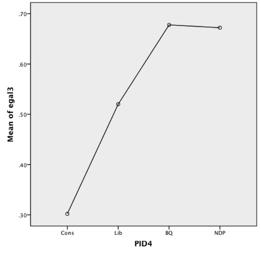
Means Plot
Interpretation
- A quick glance at the Scheffe test results in the Multiple Comparison panel indicates that in terms of Egalitarianism both Conservative and Liberal identifiers differ significantly from each of the other three partisan groups. BQ and NDP identifiers, however, do not significantly differ from one another.
- The confidence intervals provide more detail on where the significant and non-significant differences lie.
- The general hypothesis that “partisan identifiers differ in their egalitarian attitudes” is again supported by the analysis. However the one-way ANOVA test also more specifically shows that Conservatives are significantly less egalitarian in their attitudes than all other partisan groups. Moreover, Liberals while more egalitarian than Conservatives are less egalitarian than either BQ or NDP identifiers, who do not differ significantly from one another.
QUESTIONS FOR REFLECTION
- Should the results of the one-way ANOVA lead us to rethink, or reconceptualise, the relationship between partisanship and egalitarianism?
DISCUSSION
- Chi-square can tell us whether or not there are significant differences in a cross tabulation, but chi-square alone cannot tell us where those significant differences lie. In situations where more specific differences are also theoretically interesting, we can use one-way ANOVA to examine the data further and more finely tune our findings.